Why do you need a 2-NDFL certificate from your previous place of work?
Author of the question: Evseev D. Created: 02/21/22
Certificate 2-NDFL upon hiring. When applying for employment, the employer has the right to require a certificate in form 2-NDFL from the previous place of work (approved by order of the Federal Tax Service dated October 2, 2018 No. ММВ-7-11/566). The certificate is needed in order to submit standard deductions to employees with children. The fact is that an employee is entitled to a deduction only if his income for the year does not exceed 350,000 rubles. This amount is considered a cumulative total from the beginning of the year (clause 1 of Article 218 of the Tax Code of the Russian Federation). Data on income for the current year are recorded in the 2-NDFL certificate, which the previous employer
Answered by: Ovchinnikov D. 02/22/22
What is a cumulative total when calculating income tax?
The tax base for income tax is the monetary expression of the organization's profit (clause 1 of Article 274 of the Tax Code of the Russian Federation).
When determining the tax base, taxable profit is determined on an accrual basis from the beginning of the tax period (clause 7 of Article 274 of the Tax Code of the Russian Federation). Tax is calculated based on the annual base.
Advances based on the results of reporting periods are calculated based on profits calculated on an accrual basis from the beginning of the tax period to the end of the reporting period (clause 2 of Article 286 of the Tax Code of the Russian Federation). Cumulative total means that the profit of the reporting quarter is determined based on income and expenses received/incurred from the beginning of the year to the reporting date. That is, it actually includes both the profit/loss of the previous reporting period and the profit/loss of the current one.
Find out how to correctly calculate advance payments for income tax in ConsultantPlus. If you don't have access to the system, get a free trial online.
About the cumulative total in another report, read the material “6-NDFL is filled in with a cumulative total from the beginning of the year.”
How to fill out line 140 in 6 personal income tax?
Author of the question: Makarov E. Created: 02/20/22
How to fill out line 140
in calculation
6
-
personal income tax
according to the new form. In field
140
(previously
line
040) “Calculated tax amount”, reflect the amount of calculated tax at the rate from field 100 on a cumulative basis from the beginning of the year.
To determine the value of this indicator, add up the amounts of personal income tax
accrued from the income of all employees.
Answered by: Sidorova V. 02/23/22
Running Total in SQL
The running total has long been considered one of the SQL calls. Surprisingly, even after the introduction of window functions, it continues to be a bugbear (at least for beginners). Today we will look at the mechanics of 10 of the most interesting solutions to this problem - from window functions to very specific hacks. In spreadsheets like Excel, the running total is calculated very simply: the result in the first record is the same as its value:
...and then we sum the current value and the previous total.
In other words,
… or:
The appearance of two or more groups in the table complicates the task somewhat: now we calculate several totals (for each group separately). However, here too the solution lies on the surface: each time you need to check which group the current record belongs to. Click and drag
, and the job is done:
As you can see, the calculation of the cumulative total is associated with two constant components: (a)
sorting the data by date and
(b)
going back to the previous row.
But what about SQL? For a very long time it did not have the necessary functionality. The necessary tool - window functions - first appeared only in the SQL:2003
.
By this point they were already in Oracle (version 8i). But implementation in other DBMSs was delayed by 5-10 years: SQL Server 2012, MySQL 8.0.2 (2018), MariaDB 10.2.0 (2017), PostgreSQL 8.4 (2009), DB2 9 for z/OS (2007 year), and even SQLite 3.25 (2018). Test data
- creating tables and filling them with data - - the simplest case create table test_simple (dt date NULL, val int NULL ); — use the date format of our DBMS (or change the settings, for example through NLS_DATE_FORMAT in Oracle) insert into test_simple (dt, val) values ('2019-11-01', 6); insert into test_simple (dt, val) values ('2019-11-02', 3); insert into test_simple (dt, val) values ('2019-11-03', 3); insert into test_simple (dt, val) values ('2019-11-04', 4); insert into test_simple (dt, val) values ('2019-11-05', 2); insert into test_simple (dt, val) values ('2019-11-06', 4); insert into test_simple (dt, val) values ('2019-11-07', 8); insert into test_simple (dt, val) values ('2019-11-08', 0); insert into test_simple (dt, val) values ('2019-11-09', 6); insert into test_simple (dt, val) values ('2019-11-10', 0); insert into test_simple (dt, val) values ('2019-11-11', 8); insert into test_simple (dt, val) values ('2019-11-12', 8); insert into test_simple (dt, val) values ('2019-11-13', 0); insert into test_simple (dt, val) values ('2019-11-14', 2); insert into test_simple (dt, val) values ('2019-11-15', 8); insert into test_simple (dt, val) values ('2019-11-16', 7); - the case with groups create table test_groups (grp varchar NULL, - varchar2(1) in Oracle dt date NULL, val int NULL ); — we use the date format of our DBMS (or change the settings, for example, through NLS_DATE_FORMAT in Oracle) insert into test_groups (grp, dt, val) values ('a', '2019-11-06', 1); insert into test_groups (grp, dt, val) values ('a', '2019-11-07', 3); insert into test_groups (grp, dt, val) values ('a', '2019-11-08', 4); insert into test_groups (grp, dt, val) values ('a', '2019-11-09', 1); insert into test_groups (grp, dt, val) values ('a', '2019-11-10', 7); insert into test_groups (grp, dt, val) values ('b', '2019-11-06', 9); insert into test_groups (grp, dt, val) values ('b', '2019-11-07', 10); insert into test_groups (grp, dt, val) values ('b', '2019-11-08', 9); insert into test_groups (grp, dt, val) values ('b', '2019-11-09', 1); insert into test_groups (grp, dt, val) values ('b', '2019-11-10', 10); insert into test_groups (grp, dt, val) values ('c', '2019-11-06', 4); insert into test_groups (grp, dt, val) values ('c', '2019-11-07', 10); insert into test_groups (grp, dt, val) values ('c', '2019-11-08', 9); insert into test_groups (grp, dt, val) values ('c', '2019-11-09', 4); insert into test_groups (grp, dt, val) values ('c', '2019-11-10', 4); — check the data — select * from test_simple order by dt; select * from test_groups order by grp, dt;
Window functions
Window functions are probably the easiest way.
In the base case (table without groups), we are looking at data sorted by date: order by dt ... but we are only interested in the rows before the current one: rows between unbounded preceding and current row Ultimately, we need a sum with these parameters: sum(val) over (order by dt rows between unbounded preceding and current row) And the full query will look like this: select s.*, coalesce(sum(s.val) over (order by s.dt rows between unbounded preceding and current row), 0 ) as total from test_simple s order by s.dt; In the case of the cumulative total by group (field grp), we only need one small edit. Now we consider the data as divided into “windows” based on group: To account for this division, we must use the partition by keyword:
partition by grp And, accordingly, calculate the sum over these windows: sum(val) over (partition by grp order by dt rows between unbounded preceding and current row) Then the entire query is transformed in this way: select tg.*, coalesce(sum(tg .val) over (partition by tg.grp order by tg.dt rows between unbounded preceding and current row), 0) as total from test_groups tg order by tg.grp, tg.dt; The performance of window functions will depend on the specifics of your DBMS (and its version!), table sizes, and the presence of indexes. But in most cases this method will be the most effective. However, window functions are not available in older versions of the DBMS (which are still in use). In addition, they are not available in DBMSs such as Microsoft Access and SAP/Sybase ASE. If a vendor-neutral solution is needed, you should consider alternatives.
Subquery
As mentioned above, window functions were introduced very late in the major DBMSs.
This delay should not be surprising: in relational theory, data is not ordered. The solution through a subquery is much more in line with the spirit of relational theory. Such a subquery should calculate the sum of values with a date before the current one (and including the current one): .
What in code looks like this:
select s.*, (select coalesce(sum(t2.val), 0) from test_simple t2 where t2.dt <= s.dt) as total from test_simple s order by s.dt; A slightly more efficient solution would be to have a subquery count the total up to (but not including) the current date, and then sum it with the value in the row: select s.*, s.val + (select coalesce(sum(t2.val), 0) from test_simple t2 where t2.dt < s.dt) as total from test_simple s order by s.dt; In the case of a running total for several groups, we need to use a correlated subquery: select g.*, (select coalesce(sum(t2.val), 0) as total from test_groups t2 where g.grp = t2.grp and t2.dt <= g.dt) as total from test_groups g order by g.grp, g.dt; The condition g.grp = t2.grp checks whether rows are part of a group (which is basically similar to how partition by grp works in window functions).
Inner join
Since subqueries and joins are interchangeable, we can easily replace one with the other.
To do this, you need to use Self Join, joining two instances of the same table: select s.*, coalesce(sum(t2.val), 0) as total from test_simple s inner join test_simple t2 on t2.dt <= s.dt group by s.dt, s.val order by s.dt; As you can see, the filter condition in the subquery t2.dt <= s.dt has become a join condition. In addition, to use the sum() aggregation function, we need grouping by date and value group by s.dt, s.val. The same can be done for the case with different grp groups:
select g.*, coalesce(sum(t2.val), 0) as total from test_groups g inner join test_groups t2 on g.grp = t2.grp and t2.dt <= g.dt group by g.grp, g. dt, g.val order by g.grp, g.dt;
Cartesian product
Since we've replaced the subquery with a join, why not try a Cartesian product? This solution will require only minimal edits: select s.*, coalesce(sum(t2.val), 0) as total from test_simple s, test_simple t2 where t2.dt <= s.dt group by s.dt, s.val order by s.dt; Or for the case with groups: select g.*, coalesce(sum(t2.val), 0) as total from test_groups g, test_groups t2 where g.grp = t2.grp and t2.dt <= g.dt group by g .grp, g.dt, g.val order by g.grp, g.dt; The listed solutions (subquery, inner join, Cartesian join) correspond to SQL-92
and
SQL:1999
, and therefore will be available in almost any DBMS. The main problem with all these solutions is low performance. This is not a big deal if we materialize a table with the result (but we still want more speed!). Further methods are much more effective (adjusted for the already indicated specifics of specific DBMSs and their versions, table size, indexes).
Recursive query
One of the more specific approaches is a recursive query in a common table expression.
To do this, we need an “anchor” - a query that returns the very first row: select dt, val, val as total from test_simple where dt = (select min(dt) from test_simple) Then the results of the recursive query are attached to the “anchor” using union all . To do this, you can rely on the date field dt, adding one day at a time: select r.dt, r.val, cte.total + r.val from cte inner join test_simple r on r.dt = dateadd(day, 1, cte .dt) - + 1 day in SQL Server The part of the code that adds one day is not universal. For example, this is r.dt = dateadd(day, 1, cte.dt) for SQL Server, r.dt = cte.dt + 1 for Oracle, etc. By combining the “anchor” and the main query, we get the final result:
with cte (dt, val, total) as (select dt, val, val as total from test_simple where dt = (select min(dt) from test_simple) union all select r.dt, r.val, cte.total + r. val from cte inner join test_simple r on r.dt = dateadd(day, 1, cte.dt) — r.dt = cte.dt + 1 in Oracle, etc. ) select dt, val, total from cte order by dt; The solution for the case with groups will not be much more complicated: with cte (dt, grp, val, total) as (select g.dt, g.grp, g.val, g.val as total from test_groups g where g.dt = (select min(dt) from test_groups where grp = g.grp) union all select r.dt, r.grp, r.val, cte.total + r.val from cte inner join test_groups r on r.dt = dateadd(day, 1, cte.dt) - r.dt = cte.dt + 1 in Oracle, etc. and cte.grp = r.grp ) select dt, grp, val, total from cte order by grp, dt;
Recursive query with row_number() function
The previous solution relied on the continuity of the dt date field with sequential increments of 1 day. We avoid this by using the window function row_number(), which numbers rows. Of course, this is not fair - after all, we are here to consider alternatives to window functions. However, this solution may be a kind of proof of concept
: in practice, there may be a field that replaces line numbers (record id). Additionally, SQL Server introduced the row_number() function before full support for window functions (including sum()) was introduced.
So, for a recursive query with row_number(), we need two CTEs. In the first one we only number the lines:
with cte1 (dt, val, rn) as (select dt, val, row_number() over (order by dt) as rn from test_simple) ... and if the row number is already in the table, then you can do without it. In the next query we turn to cte1: cte2 (dt, val, rn, total) as (select dt, val, rn, val as total from cte1 where rn = 1 union all select cte1.dt, cte1.val, cte1.rn , cte2.total + cte1.val from cte2 inner join cte1 on cte1.rn = cte2.rn + 1 ) And the entire request looks like this: with cte1 (dt, val, rn) as (select dt, val, row_number() over (order by dt) as rn from test_simple), cte2 (dt, val, rn, total) as (select dt, val, rn, val as total from cte1 where rn = 1 union all select cte1.dt, cte1.val, cte1.rn, cte2.total + cte1.val from cte2 inner join cte1 on cte1.rn = cte2.rn + 1 ) select dt, val, total from cte2 order by dt; ... or for the case with groups: with cte1 (dt, grp, val, rn) as (select dt, grp, val, row_number() over (partition by grp order by dt) as rn from test_groups), cte2 (dt, grp , val, rn, total) as (select dt, grp, val, rn, val as total from cte1 where rn = 1 union all select cte1.dt, cte1.grp, cte1.val, cte1.rn, cte2.total + cte1.val from cte2 inner join cte1 on cte1.grp = cte2.grp and cte1.rn = cte2.rn + 1 ) select dt, grp, val, total from cte2 order by grp, dt;
CROSS APPLY/LATERAL statement
One of the most exotic ways to calculate a running total is to use the CROSS APPLY operator (SQL Server, Oracle) or the equivalent LATERAL operator (MySQL, PostgreSQL).
These operators appeared quite late (for example, in Oracle only from version 12c). And in some DBMSs (for example, MariaDB) they don’t exist at all. Therefore, this decision is of purely aesthetic interest. Functionally, using CROSS APPLY or LATERAL is identical to a subquery: we append the calculation result to the main query:
cross apply (select coalesce(sum(t2.val), 0) as total from test_simple t2 where t2.dt <= s.dt ) t2 ... which looks like this: select s.*, t2.total from test_simple s cross apply (select coalesce(sum(t2.val), 0) as total from test_simple t2 where t2.dt <= s.dt ) t2 order by s.dt; The solution for the case with groups will be similar: select g.*, t2.total from test_groups g cross apply (select coalesce(sum(t2.val), 0) as total from test_groups t2 where g.grp = t2.grp and t2 .dt <= g.dt ) t2 order by g.grp, g.dt; Total: we looked at the main platform-independent solutions. But there remain solutions specific to specific DBMSs! Since there are so many possible options here, we will focus on a few of the most interesting ones.
MODEL Statement (Oracle)
The MODEL statement in Oracle provides one of the most elegant solutions.
At the beginning of the article, we looked at the general formula for the cumulative total: MODEL allows you to implement this formula literally one to one! To do this, we first fill the total field with the values of the current row
select dt, val, val as total from test_simple ... then calculate the row number as row_number() over (order by dt) as rn (or use a ready-made number field, if available). And finally, we introduce a rule for all lines except the first: total = total[cv() - 1] + val[cv()].
The cv() function here is responsible for the value of the current line. And the whole request will look like this:
select dt, val, total from (select dt, val, val as total from test_simple) t model dimension by (row_number() over (order by dt) as rn) measures (dt, val, total) rules (total = total[ cv() - 1] + val[cv()]) order by dt;
Cursor (SQL Server)
The cumulative total is one of the few cases where the cursor in SQL Server is not only useful, but also preferable to other solutions (at least until version 2012, where window functions were introduced).
The implementation via a cursor is quite trivial. First you need to create a temporary table and fill it with dates and values from the main one:
create table #temp (dt date primary key, val int NULL, total int NULL ); insert #temp (dt, val) select dt, val from test_simple order by dt; Then we set local variables through which the update will occur: declare @VarTotal int, @VarDT date, @VarVal int; set @VarTotal = 0; After this, we update the temporary table through the cursor: declare cur cursor local static read_only forward_only for select dt, val from #temp order by dt; open cur; fetch cur into @VarDT, @VarVal; while @@fetch_status = 0 begin set @VarTotal = @VarTotal + @VarVal; update #temp set total = @VarTotal where dt = @VarDT; fetch cur into @VarDT, @VarVal; end; close cur; deallocate cur; And finally, we get the desired result: select dt, val, total from #temp order by dt; drop table #temp;
Update via local variable (SQL Server)
Updating via a local variable in SQL Server is based on undocumented behavior and should not be considered reliable.
Nevertheless, this is perhaps the fastest solution, and this is why it is interesting. Let's create two variables: one for cumulative totals and a table variable:
declare @VarTotal int = 0; declare @tv table (dt date NULL, val int NULL, total int NULL ); First, fill @tv with data from the main table insert @tv (dt, val, total) select dt, val, 0 as total from test_simple order by dt; Then we update the table variable @tv using @VarTotal: update @tv set @VarTotal = total = @VarTotal + val from @tv; ... after which we get the final result: select * from @tv order by dt; Summary: we looked at the top 10 ways to calculate a running total in SQL. As you can see, even without window functions this problem is completely solvable, and the mechanics of the solution cannot be called complex.
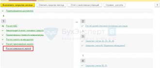
How can I see profit or loss using OS?
Author of the question: Veselov I. Created: 02/21/22
In order to see the profit, you need to generate SALT for account 99.01 for the required period. The turnover on the credit of the account is the profit received during the period, the turnover on the debit is the loss. The balance at the end of the period is the profit or loss obtained at the end of the period. The financial result is formed on an accrual basis from the beginning of the year. On December 31, the balance sheet is reformed, and the accumulated balance on account 99.01 is written off to account 84 (retained profit/uncovered loss).
Answered by: Danilova B. 02/23/22
Making advance payments
After calculating advance payments based on previous periods, the company is obliged to transfer the advance payment for each month of the current quarter no later than the 28th. When the reporting period ends - in our case, a quarter - the tax is calculated from the actual profitability indicators. If, after deducting advances, there is an underpayment, it is paid additionally.
Monthly advance payments are transferred by the 28th day of the month following the reporting month. You must pay for January by February 28, February by March 28, etc. The last payment for December–January is due by March 28 of the following year.
Quarterly payments are transferred by the 28th day of the month after the end of the reporting quarter. For example, for the 1st quarter until April 28, the 2nd and 3rd quarters - until July 28 and October, respectively. The final payment for the year must be completed by March 28 of the following year.
Newly created organizations can pay once a quarter - according to the third scheme. A company is considered new for four quarters after its creation. Subject to compliance with the minimum profit limit of 5 million rubles. per month, the company may not make monthly advance payments. The second condition, specified in Art. 287, clause 5 of the Tax Code of the Russian Federation for such organizations - profit no more than 15 million per quarter.